The Power of Recursion: Unveiling Hidden Connections and Patterns

When implementing recursion, it is crucial to ensure that the recursive calls converge towards the base case. If the recursive calls do not eventually reach the base case, the recursion will continue indefinitely, leading to a stack overflow or infinite loop.
Recursion and Function Stack
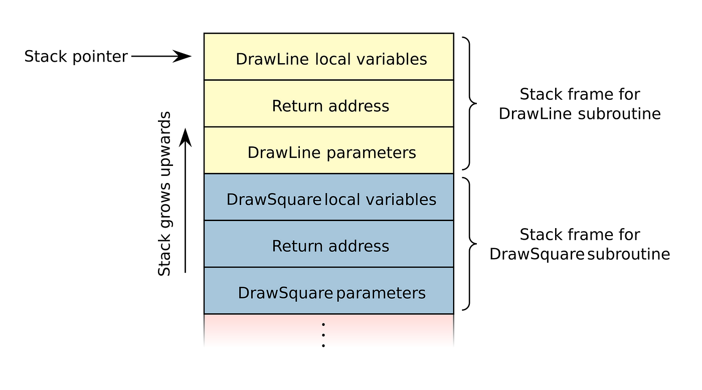 Call Stack for Functions (source: Wikipedia)
Recursion and the function stack are closely intertwined concepts in computer programming. When a recursive function is called, it creates a sequence of nested function calls, each adding a new frame to the function stack. The function stack, also known as the call stack or execution stack, keeps track of the active function calls and their associated data.
Let’s explore the relationship between recursion and the function stack in more detail:
Recursive Function Calls
When a recursive function is invoked, it typically performs two main actions:
— Checks for a base case: The base case represents the simplest form of the problem that can be directly solved without further recursion. If the base case is met, the function returns a value or performs a specific action.
— Makes a recursive call: If the base case is not met, the function calls itself with modified parameters or arguments to solve a smaller subproblem. This recursive call creates a new frame on top of the function stack.
Function Stack
The function stack is a data structure used by the programming language to keep track of function calls and their associated information. Each time a function is called, a new frame is added to the top of the stack, containing the function’s parameters, local variables, and the return address — the point in the code where the function was called from.
Recursive Depth and Unwinding
As recursive function calls are made, the function stack grows in depth, with each new call adding a new frame to the stack. This depth represents the number of recursive function calls that are currently active. When the base case is reached, the recursion starts unwinding. The function stack is gradually reduced as each function call returns its result and removes its frame from the stack. This unwinding process continues until the initial function call (the first one made) returns, resulting in an empty function stack.
Stack Overflow
It is essential to handle recursion carefully to prevent stack overflow errors. If the base case is not properly defined or the recursive calls do not converge towards the base case, the function stack can grow infinitely, exhausting the available memory and causing a stack overflow. This usually results in a runtime error and program termination.
Why Function Stack?
Understanding the function stack and its relationship with recursion is crucial for designing and debugging recursive algorithms. It helps programmers trace the execution flow, track variable values at each recursive level, and identify any issues related to stack overflow or incorrect termination conditions.
This is the essence of the relation between function stack and recursion: it waits until all the children of the previous line’s function call are finished before running the next line in the call stack.
Recursion Implementation in Python (Basic to Expert)
Basic Implementation: Factorial
Here’s an example of recursion in code using the Python programming language. Let’s consider a classic example: calculating the factorial of a number.
def factorial(n):
    # Base case: factorial of 0 or 1 is 1
    if n == 0 or n == 1:
        return 1
    else:
      # Recursive step: multiply n by the factorial of (n-1)
      return n * factorial(n - 1)

# Testing the factorial function
number = 5
result = factorial(number)
print(f"The factorial of {number} is: {result}")
The output of the code will be:
The factorial of 5 is: 120
In this example, the `factorial` function takes an integer `n` as an input and computes its factorial using recursion.
At the beginning of the function, we define a base case to handle the simplest case: when `n` is either 0 or 1. In such cases, the factorial is defined as 1. This provides the termination condition for the recursion.
For other values of `n`, the function enters the recursive step. It calls itself with the argument `(n — 1)` and multiplies it by `n`. This recursive call continues until the base case is reached, and then the function starts unwinding, returning the intermediate results and eventually providing the final factorial value.
In the example, we calculate the factorial of 5. The `factorial` function is called with `number` as the argument, and the result is stored in the `result` variable. Finally, we print the factorial value using f-string formatting.
The recursive approach elegantly breaks down the problem of calculating the factorial into smaller subproblems until the base case is reached, resulting in an efficient solution.
Function Stack
Let’s visualize the function stack for the `factorial` function when called with `n = 5`:
factorial(5)
├─ factorial(4)
│ ├─ factorial(3)
│ │ ├─ factorial(2)
│ │ │ ├─ factorial(1)
│ │ │ │ └─ factorial(0) => returns 1
│ │ │ └─ returns 2 * factorial(1) => returns 2
│ │ └─ returns 3 * factorial(2) => returns 6
│ └─ returns 4 * factorial(3) => returns 24
└─ returns 5 * factorial(4) => returns 120
In the visualization above, each indented line represents a function call, and the arrow (`=>`) indicates the return value of that particular function call. The `factorial` function recursively calls itself, reducing the input `n` by 1 in each recursive step until it reaches the base case (`n == 0` or `n == 1`), where it returns 1. As the function calls return their values, the function stack unwinds, resulting in the final factorial value of the original input.
The visualization demonstrates the build-up of the function stack as each recursive call is made, and subsequent calls are nested within each other. As the recursive calls reach the base cases, the function calls start returning their values, unwinding the stack and propagating the results back to the original call.
Variation 1 || Double Recursion Implementation : Fibonacci Numbers
Here’s an example of double recursion in code using Python. Let’s consider a common problem: calculating the Fibonacci sequence.
def fibonacci(n):
 # Base cases: Fibonacci of 0 is 0, Fibonacci of 1 is 1
 if n == 0:
 return 0
 elif n == 1:
 return 1
 else:
 # Recursive step: Fibonacci of n is the sum of the previous two Fibonacci numbers
 return fibonacci(n - 1) + fibonacci(n - 2)
# Testing the fibonacci function
number = 6
result = fibonacci(number)
print(f"The Fibonacci number at position {number} is: {result}")
The output of the code will be:
The Fibonacci number at position 6 is: 8
In this example, the `fibonacci` function takes an integer `n` as an input and computes the Fibonacci number at that position using double recursion.
Similar to the previous example, we define base cases to handle the simplest cases: when `n` is 0 or 1. In these cases, the Fibonacci number is defined as 0 and 1, respectively.
For other values of `n`, the function enters the recursive step. It calls itself twice, with the arguments `(n — 1)` and `(n — 2)`, respectively, and then adds the results of these two recursive calls. This is because each Fibonacci number is the sum of the previous two Fibonacci numbers. The recursive calls continue until the base cases are reached, and then the function starts unwinding, returning the intermediate results and eventually providing the Fibonacci number at position `n`.
In the example, we calculate the Fibonacci number at position 6. The `fibonacci` function is called with `number` as the argument, and the result is stored in the `result` variable. Finally, we print the Fibonacci number using f-string formatting.
Double recursion allows us to break down the problem of finding the Fibonacci number at a specific position by recursively calling the function with `(n — 1)` and `(n — 2)`, creating a branching tree of recursive calls. This approach efficiently computes the desired Fibonacci number.
Function Stack
Let’s visualize the function stack for the fibonacci function when called with the argument number = 6:
fibonacci(6)
├─ fibonacci(5)
│   ├─ fibonacci(4)
│   │   ├─ fibonacci(3)
│   │   │   ├─ fibonacci(2)
│   │   │   │   ├─ fibonacci(1)
│   │   │   │   └─ fibonacci(0)
│   │   │   └─ fibonacci(1)
│   │   └─ fibonacci(2)
│   │       ├─ fibonacci(1)
│   │       └─ fibonacci(0)
│   └─ fibonacci(3)
│       ├─ fibonacci(2)
│       │   ├─ fibonacci(1)
│       │   └─ fibonacci(0)
│       └─ fibonacci(1)
└─ fibonacci(4)
    ├─ fibonacci(3)
    │   ├─ fibonacci(2)
    │   │   ├─ fibonacci(1)
    │   │   └─ fibonacci(0)
    │   └─ fibonacci(1)
    └─ fibonacci(2)
        ├─ fibonacci(1)
        └─ fibonacci(0)
In the visualization above, each indented line represents a function call, and the arrow (└─) indicates the return value of that particular function call. As we can see, the fibonacci function recursively calls itself, diving deeper into smaller subproblems until it reaches the base cases (n == 0 and n == 1), where it returns the corresponding Fibonacci numbers.
Notice how in the visualization, the children of fibonacci(6) are fibonacci(5) and fibonacci(4). But fibonacci(4) does not start immediately after fibonacci(5), instead it waits until all children of fibonacci(5) and its subsequent function stack children is done. This is the essence of the relation between function stack and recursion: it waits until all the children of the previous line’s function call are finished before running the next line in the call stack.ü
Variation 2 || Mutual Recursion: Even and Odd
Mutual recursion refers to a situation where two or more functions are defined in terms of each other, creating a circular dependency. Each function calls the other(s) in a cyclical manner, allowing them to work together to solve a problem.
Here’s an example of mutual recursion using Python:
def is_even(n):
 if n == 0:
 return True
 else:
 return is_odd(n - 1)
def is_odd(n):
 if n == 0:
 return False
 else:
 return is_even(n - 1)
# Testing the mutual recursion
number = 4
print(f"Is {number} even? {is_even(number)}")
print(f"Is {number} odd? {is_odd(number)}")
The output of the code will be:
Is 4 even? True
Is 4 odd? False
In this example, we have two functions: `is_even` and `is_odd`. They rely on each other to determine whether a given number is even or odd.
The `is_even` function checks if the number `n` is equal to 0. If it is, it returns `True`, indicating that the number is even. Otherwise, it calls the `is_odd` function with the argument `(n — 1)`. This mutual recursion allows the functions to work together, with `is_odd` taking over the evaluation to determine if the number is odd.
Similarly, the `is_odd` function checks if the number `n` is equal to 0. If it is, it returns `False`, indicating that the number is not odd. Otherwise, it calls the `is_even` function with the argument `(n — 1)`.
In the example, we use the mutual recursion by checking whether the number 4 is even or odd. We call both functions with the number as an argument and print the results using f-string formatting.
Mutual recursion allows functions to delegate parts of their computation to each other, effectively dividing the problem into smaller parts that can be solved collectively. It can be a powerful technique for organizing complex code and solving problems that naturally exhibit circular dependencies.
Function Stack
Let’s visualize the function stack for the mutual recursion between the is_even and is_odd functions when called with number = 4:
is_even(4)
└─ is_odd(3)
   └─ is_even(2)
      └─ is_odd(1)
         └─ is_even(0) => returns True
      └─ returns True
   └─ returns True
└─ returns True
In the visualization above, each indented line represents a function call. The mutual recursion occurs between the is_even and is_odd functions. The is_even function checks if the number is divisible by 2, while the is_odd function checks if the number is not divisible by 2. In this example, is_even(4) is the initial call. It invokes the is_odd function with n = 3, which, in turn, invokes the is_even function with n = 2. This mutual recursion continues until the base case is reached. Eventually, the is_even(0) call is reached, which returns True. This value is then propagated back through the function calls until it reaches the original call to is_even(4).
Applications in Computer Science
Recursion finds extensive use in computer science, offering powerful techniques for solving various problems. One classic example is the computation of factorials. The factorial of a positive integer “n” (denoted as “n!”) is the product of all positive integers from 1 to “n.” By expressing the factorial recursively, we can define it as the product of “n” and the factorial of “n-1” until we reach the base case of 1.
Another prominent application lies in recursive algorithms such as quicksort and mergesort, which efficiently sort large datasets by repeatedly dividing them into smaller subproblems and combining the results.
Recursion is also widely utilized in data structures like trees and graphs. Tree traversal algorithms, such as depth-first search and breadth-first search, employ recursion to explore the hierarchical structure of a tree, enabling efficient searching, manipulation, and analysis.
Beyond Computer Science
While recursion is commonly associated with computer science, its influence extends beyond the realm of programming. The concept of recursion finds applications in linguistics, where self-embedding sentences and recursive grammatical structures provide intriguing insights into the nature of human language.
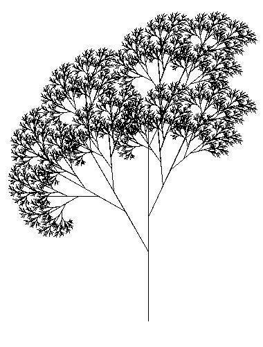
Recursion has also made significant contributions in mathematics, specifically in number theory and fractal geometry. In number theory, the Fibonacci sequence, a series of numbers where each term is the sum of the two preceding ones, is often defined recursively. Fractals, characterized by self-similarity, exemplify recursive patterns at varying scales and have captivated mathematicians and artists alike.
The Mind-Blowing Infinite
One of the mesmerizing aspects of recursion is its ability to evoke the infinite. By recursively calling a function, each subsequent call nests deeper into the previous one, creating an unbounded sequence of operations that can theoretically continue forever. This recursive depth is limited only by the constraints of the computing system or the resources available.