Data engineering at Meta: High-Level Overview of the internal tech stack

This article provides an overview of the internal tech stack that we use on a daily basis as data engineers at Meta. The idea is to shed some light on the work we do, and how the tools and frameworks contribute to making our day-to-day data engineering work more efficient, and to share some of the design decisions and technical tradeoffs that we made along the way.
The data warehouse
What we call the data warehouse is Meta’s main data repository that is used for analytics. It is distinct from the live “graph database” (TAO) which is used for serving content to users in real time. It is a collection of millions of Hive tables, physically stored using an internal fork of ORC (which you can read more about here). Our exabyte-scale data warehouse (one exabyte is 1,000,000 terabytes) is so large that it cannot physically be stored in one single datacenter. Instead, data is spread across different geographical locations.
Since the warehouse is not physically located in one single region, it is split into “namespaces”. Namespaces correspond to both a physical (geographical) and logical partitioning of the warehouse: tables that correspond to a similar “theme” are grouped together in the same namespace, so that they can be used in the same queries efficiently, without having to transfer data across locations.
If there’s the need to use tables from two different namespaces in a query (eg: table1 in namespace A and table2 in namespace B), then we need to replicate data: either we can choose replicate table2 to namespace A, or we replicate table1 to namespace B. We can then run our query in the namespace where both tables exist. Data engineers can create these cross-namespace replicas in a few minutes through a web-based tool, and they will automatically be kept in sync.
While namespaces partition the entire warehouse, tables are also themselves partitioned. Almost all tables in the warehouse have a ds partition column (ds for datestamp in YYYY-MM-DD format), which is generally the date at which the data was generated. Tables can also have additional partition columns to improve efficiency, and each individual partition is stored in a separate file for fast indexing.
Data is only retained in Meta’s systems for the period of time needed to fulfill the purpose for which the data was collected. Tables in the warehouse almost always have finite retention, which means that partitions older than the table’s retention time (e.g. 90 days) will automatically either be archived (anonymized and moved to a cold storage service) or deleted.
All tables are associated with an oncall group, which defines which team owns this data, and who users should refer to if they encounter an issue or have a question on the data in that table.
How is data written into the warehouse?
The three most common ways data is written into the warehouse are:
- Data workflows and pipelines, e.g. data that gets inserted by a Dataswarm pipeline (more details about that below), generally obtained by querying other tables in the warehouse,
- Logs, e.g. data that results from either server-side or client-side logging frameworks.
- Daily snapshots of entities in the production graph database.
Data discovery, data catalog
When dealing with such a huge warehouse, finding the data needed for analysis can seem like trying to find a needle in a haystack. Thankfully, engineers at Meta developed a web-based tool called iData, in which users can simply search by keyword. iData will then find and display the most relevant tables for that keyword. It is a search engine for the data warehouse: iData ranks search results in an intelligent way that generally finds you the table that you were looking for in the top results.
To display the best results, it takes into account several features of each table: data freshness, documentation, number of downstream usages (in ad hoc queries, other pipelines or dashboards — typically, a table that is used in many places can be seen as more reliable), the number of mentions in internal Workplace posts, the number of tasks associated to it, etc.
It can also be used to do advanced searches, e.g. search for tables that contain specific columns, that are assigned to a particular oncall group, and so on.
iData can be used to find other types of data assets in addition to tables (such as dashboards), and also includes lineage tools to explore upstream and downstream dependencies of any asset. This makes it possible to quickly determine what pipelines are used to produce data for high-level dashboards and what logging tables sit upstream of those.
Presto and Spark: Querying the warehouse
The warehouse can be queried by many different entry points, but data engineers at Meta generally use Presto and Spark. While both are open-source (Presto was originally developed at Meta and was open-sourced in 2019), Meta uses and maintains its own internal forks — but frequently rebases from the open-source repository so that we’re kept up-to-date, and contributes features back into the open-source projects.
With our focus primarily on business impact, design and optimization, most of our pipelines and queries are written in SQL in one of two dialects (Spark SQL or Presto SQL). Although we also leverage Spark’s Java, Scala, and Python APIs to generate and manage complex transformations for greater flexibility. This approach provides a consistent understanding of the data and business logic and enables any data engineer, data scientist, or software engineer comfortable with SQL to understand all of our pipelines and even write their own queries. More importantly, understanding the data and its lineage helps us comply with the myriad of privacy regulations.
The choice of Presto or Spark depends mostly on the workload: Presto is typically more efficient and is used for most queries while Spark is employed for heavy workloads that require higher amounts of memory or expensive joins. Presto clusters are sized in a way that most day-to-day adhoc queries (that scan, generally, a few billions rows — which is considered a light query at Meta scale) produce results in a few seconds (or minutes, if there’s complex joins or aggregations involved).
Scuba: Real-time analytics
Scuba is Meta’s real-time data analytics framework. It is frequently used by data engineers and software engineers to analyze trends on logging data in real time. It is also extensively used for debugging purposes by software and production engineers.
Scuba tables can be queried either through the Scuba web UI (which is comparable to tools like Kibana), or via a dialect of SQL. In the Scuba web UI, engineers can quickly visualize trends on a log table without having to write any queries, with data that was generated in the past few minutes.
Data that lives in Scuba often comes directly from client-side or server-side logs, but Scuba can also be used to query the results of data pipelines, real-time stream processing systems, or other systems. Each source can be configured to store a sampled percentage of the data into Scuba. Loggers are typically configured to write 100% of their rows to Hive, but a smaller percentage to Scuba as it’s more expensive to ingest and store data.
Daiquery & Bento: Query and analysis notebooks
Daiquery is one of the tools data engineers use on a daily basis at Meta. It is a web-based notebooks experience which acts as a single entrypoint to query any data source: the warehouse (either through Presto or Spark), Scuba, and plenty of others. It includes a notebook interface with multiple query cells, and users can quickly run and iterate on queries against our data warehouse. Results appear as tables by default, but built-in visualization tools allow the creation of many different types of plots.
Daiquery is optimized for rapid query development, but doesn’t support more complex post-query analysis. For this, users can promote their Daiquery notebooks into Bento notebooks. Bento is Meta’s internal implementation of managed Jupyter notebooks, and in addition to queries also enables python or R code (with a range of custom kernels for different use cases) and access to a wide range of visualization libraries. In addition to its use by data engineers, Bento is also used extensively by data scientists for analytics and machine learning engineers for running experiments and managing workflows.
Unidash: Dashboarding
Unidash is the name of the internal tool data engineers use to create dashboards (similar to Apache Superset or Tableau). It integrates with Daiquery (and many other tools): for example, engineers can write their query in Daiquery, create their graph there, and then export it to a new or existing Unidash dashboard.
Our dashboards typically show a highly-aggregated view of the underlying data. Running a query to aggregate the underlying data each time the dashboard is loaded is often prohibitively expensive. In many cases data engineers can work around this by writing pipelines to pre-aggregate data to an appropriate level for the dashboard, but in some cases this is not possible due to the complexity of the dashboard itself. To help with these cases, our internal Presto implementation includes an extension called RaptorX which caches commonly-used data and can provide as much as a 10x speedup for time-critical queries.
Most Unidash dashboards are created through a web interface which allows for quick iteration and interactive development. Unidash dashboards can also be created via a python API which allows dashboards to more easily scale to higher complexities and makes it easier for dashboard changes to be reviewed (at the cost of a more involved initial setup).
Software development
Data engineers develop pipelines to produce critical datasets to enable decision making through the use of tools like Daiquery and Unidash, data engineers at Meta also write code to define data pipelines, interface with internal systems, create team-specific tools, contribute to company-wide data infrastructure tools, and similar.
Most engineers at Meta use a highly customized version of Visual Studio Code as an IDE to work on our pipelines. It includes plenty of custom plugins, developed and maintained by internal teams. We use an internal fork of Mercurial for source control (recently open-sourced as Sapling), and a near-monorepo structure — all data pipelines and most internal tools at Meta are in a single repository with logger definitions and configuration objects in two other repositories.
Writing pipelines
Data pipelines are mostly written in SQL (for business logic), wrapped in Python code (for orchestration and scheduling).
The Python library we use for orchestrating and scheduling pipelines is internally known as Dataswarm. It is a predecessor to Airflow, and is developed and maintained internally. If you wish to learn more about the inner workings of Dataswarm, one of the software engineers who worked on Dataswarm made a great presentation about it in 2014, which is available on YouTube. While the framework has evolved since then, the base principles in that presentation are still relevant to this day.
Pipelines are built on blocks called “operators”. The pipeline is a directed acyclic graph (DAG), and each operator is a node in the DAG.
Many operators are available in Dataswarm, they can be divided in a few main categories:
- WaitFor operators, a type of operator that waits for something to happen (typically, a partition in a specific upstream table to be landed in the warehouse),
- Query operators, to run a query on an engine (typically either Presto or Spark for querying the warehouse),
- Data quality operators, to execute automated checks on the inserted data in a table,
- Data transfer operators, to transfer data between systems,
- Miscellaneous operators (e.g.: sending an email, pinging someone through chat, calling an API, executing a script…)
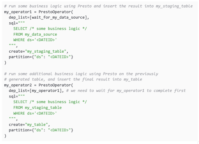
The code to define a simple pipeline looks something like this: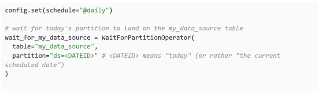
 Our internal VSCode extensions process the pipeline definition on save and calculate the DAG:
If there is an error in any of the SQL statements, the custom linter will display a warning before even trying to run the pipeline. The same extensions also allow the data engineers to schedule a test run of the new version using real input data, writing the output to a temporary table.
UPM: Advanced pipeline features
If you re-read the code above, you may notice some redundancies. In this example, we ask the first operator to wait for today’s partition to land for my_data_source, and in the second operator, we ask the framework to wait for my_operator1, because we need the <DATEID> partition to exist in my_staging_table. But we can somewhat already infer this just by looking at the SQL query: WHERE ds=’<DATEID>’ implies that we depend on the <DATEID> partition for this table. And, as engineers, we don’t like to repeat ourselves.
A team of engineers at Meta tackled this problem and built a framework called Unified Programming Model (UPM), which does exactly this: when used in a Dataswarm pipeline it parses SQL queries in the operators and correctly infer which partitions each operator needs to wait for. (Note that this is only one feature provided by UPM which will be covered in more detail in the “Future of data engineering” post series). With the use of UPM, all of the “WaitFors” and dependencies can be automatically inferred. The pipeline code can then be reduced to its core business logic: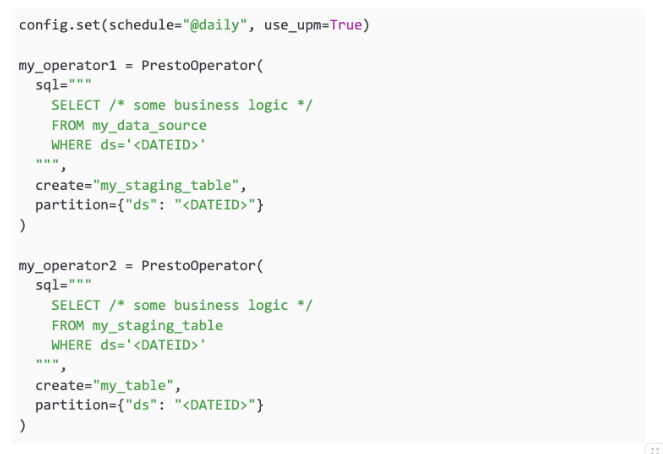 In general though, the data engineer writing the pipeline will verify that the dependencies inferred by UPM are correct, by looking at the generated DAG.
Analytics Libraries
In addition to simplifying the development of pipelines, UPM and other analytics libraries are also used to generate certain types of complex pipelines (such as for growth accounting or retention) which are unwieldy to create by hand. These libraries produce pipelines following common patterns using customizations provided by the user.
One simple example is to produce a digest-style table (which will be discussed in detail in a future blog post).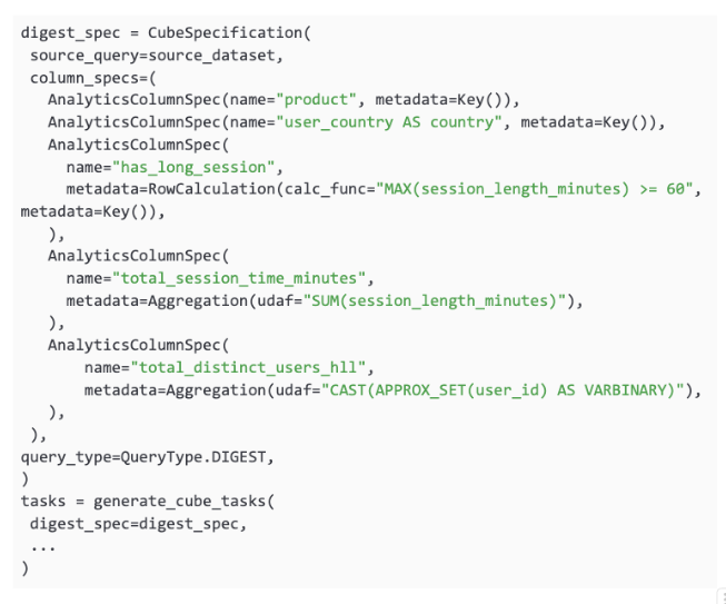 This produces a table with three dimension columns (product, country and has_log_session) and two aggregate metric columns, total_session_time_minutes and total_distinct_users_hll. This last column uses the HyperLogLog type in Presto which is used for approximate counting.
Monitoring & operations
Pipeline monitoring is done via a web-based tool called CDM (Central Data Manager), which can be seen as the Dataswarm UI.Screenshot of the CDM tool (tasks were renamed)
This view is similar to Airflow’s Tree View, but this is the entrypoint to a broader tool which allows us to:
- Quickly identify failing tasks, and find the corresponding logs
- Define and run backfills
- Navigate to upstream dependencies (e.g. for a waitfor, it will navigate to the pipeline that generated the upstream table that we’re waiting for)
- Identify upstream blockers (CDM will navigate through the recursive upstream dependencies, and automatically find the root cause of a stuck pipeline)
- Enable notifications and escalations if partitions do not land according to a configured SLA
- Set up and monitor data quality checks
- Monitor in-flight tasks and historic performance
Conclusion
This article provides an overview of the tools and systems most commonly used by data engineers, but there’s a lot of variation across the company. Some data engineers focus primarily on developing pipelines and creating dashboards, but others focus on logging, develop new analytical tools, or focus entirely on managing ML workloads.
This article doesn’t include a few important tools and systems which are worth a deeper look and will be covered in future blog posts:
- Tools for managing metrics and experiments
- Our experimental testing platform
- Tools for managing experiment exposures and rollouts
- Privacy tools
- Specialized tools for managing ML workloads
- Operational Tooling for understanding metric movements
Our data warehouse and systems have grown and changed to meet the needs of the company, and as such are constantly evolving to support new needs. Our ongoing work includes expanding our privacy-aware infrastructure, reducing the cost of queries and the amount of data that we keep in storage, and making it easier for data engineers to manage large suites of pipelines. Overall these changes help reduce the amount of repetitive work performed by data engineers, allowing them to spend more time focusing on product needs.